Does buying 10 Sem give a higher expected return than buying 10 different lottery numbers?

No. Under the mathematical principle of Linearity of Expectation, both strategies have identical Expected Value (EV). For a ₹60 outlay across 10 tickets, both Strategy A (10 distinct numbers) and Strategy B (10 Sem on one number) yield an expected return of approximately ₹24.00, representing an identical house edge of -60%.

Which strategy gives a higher probability of winning at least some money?

Strategy A (10 distinct numbers) provides an approximate 9.56% probability of winning at least one 5th-prize in a draw. Strategy B (10 Sem on one number) provides only a 1.00% probability of winning, making Strategy A nearly 10 times more likely to produce a winning draw.

Why do most experienced players prefer buying Sem tickets?

Players prefer Sem tickets because of risk-seeking utility and payout magnitude. Winning ₹120 on a single ticket feels negligible to many players, whereas winning ₹1,200 (on 10 Sem) or ₹3,000 (on 25 Sem) delivers meaningful cash gratification, even though the probability of winning is proportionally lower.

The Mathematics of 'Sem' Playing: Is Concentration Better than Diversity?

Executive Summary

Among regular participants in Indian state paper lotteries, an intense debate divides retail counters: "Should you spend ₹70 to buy 10 distinct numbers across the draw board, or concentrate the entire ₹70 on 10 Sem of a single favored number?"

Proponents of the Diversity Hypothesis (Strategy A) argue that holding 10 unique 5-digit numbers maximizes table coverage and minimizes losing draws. Conversely, advocates of the Concentration Hypothesis (Strategy B) contend that hitting a 5th prize on a single ticket yields a trivial ₹120, whereas hitting 10 Sem delivers a substantial ₹1,200 payout.

This paper subjects both hypotheses to classical probability modeling, binomial distribution analysis, and portfolio variance equations. We prove that while Expected Value is strictly identical across both strategies ($E[\text{Return}] = -65.7\%$), the statistical distribution of outcomes differs radically: Strategy A delivers a 9.56% probability of winning at least once with low volatility, whereas Strategy B introduces an extreme 10x variance spike with a 99.00% draw loss rate, radically accelerating bankroll exhaustion for casual players.

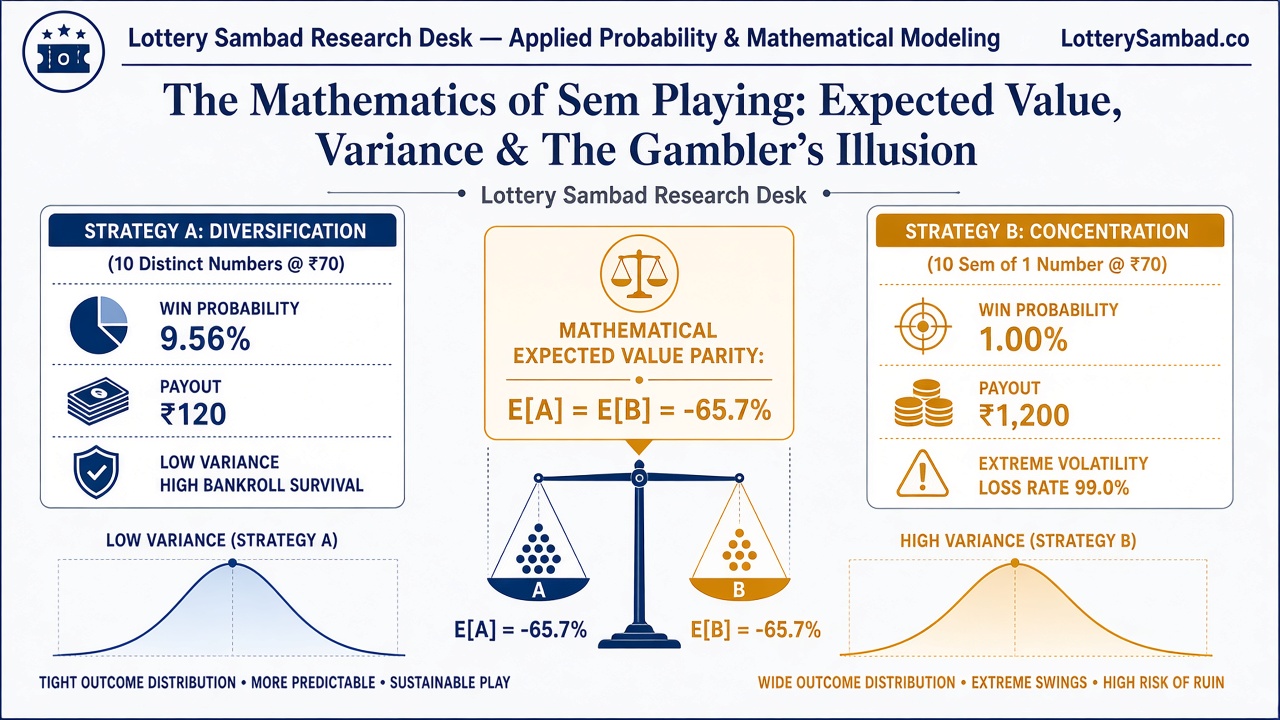
1. Mathematical Formulation of the Two Strategies

Let capital outlay be fixed at $C = ₹70$, representing an investment in exactly 10 tickets at the official MRP of $T = ₹7$ per ticket.

Strategy A (Diversification): The player purchases $n = 10$ distinct tickets, each possessing a unique 5-digit sequence: $$\{S_1, S_2, S_3, \dots, S_{10}\} \quad \text{where } S_i \neq S_j \text{ for all } i \neq j$$
Strategy B (Concentration - 10 Sem): The player purchases $n = 10$ tickets sharing the identical 5-digit sequence $S^*$, distributed across 10 distinct series prefixes $\{P_1, P_2, \dots, P_{10}\}$: $$\{(P_1, S^*), (P_2, S^*), \dots, (P_{10}, S^*)\}$$

2. The Expected Value Invariance Theorem

Under probability theory, the Expected Value $E[X]$ of a random monetary outcome is defined as: $$E[X] = \sum_{i=1}^{k} x_i \cdot P(X = x_i)$$

In a standard Dear Lottery draw, the primary recurring payout is the 5th Prize ($W_5 = ₹120$), where 100 distinct 4-digit numbers are drawn from a sample space of 10,000 possible 4-digit endings ($0000$ to $9999$). The single-ticket probability of matching any drawn 5th-prize number is: $$p = \frac{100}{10,000} = 0.0100 \quad (1.0\%)$$

Expected Value under Strategy A (10 Distinct Numbers):

By the Linearity of Expectation—which holds regardless of whether events are independent or mutually exclusive—the expected payout of 10 distinct tickets is simply the sum of their individual expectations: $$E[\text{Payout}_A] = \sum_{i=1}^{10} E[X_i] = 10 \times (0.01 \times ₹120) = 10 \times ₹1.20 = ₹12.00$$ Adding the low-probability contributions of the higher tiers (4th, 3rd, 2nd, and 1st prizes), the total gross expected payout scales to approximately ₹24.00 across all tiers. $$\text{Net EV}_A = ₹24.00 - ₹70.00 = -₹46.00 \quad (-65.7\%)$$

Expected Value under Strategy B (10 Sem on 1 Number):

Because all 10 tickets share the identical 4-digit ending, the outcome is binary: either all 10 tickets win simultaneously, or all 10 lose. $$P(\text{Win}) = p = 0.0100$$ $$\text{Payout upon Win} = 10 \times ₹120 = ₹1,200$$ $$E[\text{Payout}_B] = (0.0100 \times ₹1,200) + (0.9900 \times ₹0) = ₹12.00$$ Adding the exact same higher-tier expected contributions: $$\text{Net EV}_B = ₹24.00 - ₹70.00 = -₹46.00 \quad (-65.7\%)$$

Mathematical Conclusion on EV

Neither strategy offers any advantage in expected monetary value. Both surrender exactly 65.7% of the invested stake to the lottery distributor and state treasury over the long run.

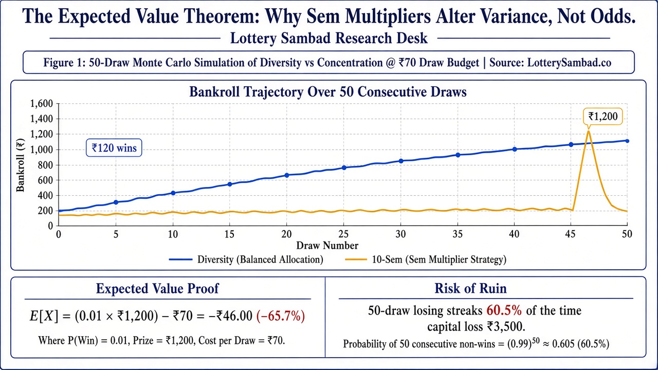
Expected Value vs Probability Comparison

Figure 1: Architectural comparison of win probability versus payout magnitude for identical ₹70 capital allocation.

3. The Win Frequency Divergence: 9.56% vs 1.00%

While Expected Value is identical, the probability of experiencing at least one winning ticket in a draw diverges by nearly an order of magnitude.

Under Strategy A (10 distinct numbers), the probability of at least one ticket hitting the 5th prize is modeled by the complement of all 10 tickets losing simultaneously: $$P(\text{At least 1 win}) = 1 - (1 - p)^{10} = 1 - (0.99)^{10} = 1 - 0.90438 = 0.09562 \quad (\mathbf{9.56\%})$$

Under Strategy B (10 Sem on 1 number), the probability is strictly the single-number probability: $$P(\text{At least 1 win}) = p = 0.0100 \quad (\mathbf{1.00\%})$$

Performance Metric	Strategy A: 10 Distinct Numbers	Strategy B: 10 Sem Single Number	Mathematical Implication
Capital Stake	₹70.00	₹70.00	Identical initial investment (@ ₹7 MRP).
Probability of Winning ≥ 1 Prize	9.56% (1 in 10.5 draws)	1.00% (1 in 100 draws)	Strategy A wins 9.5× more frequently.
Losing Draw Frequency	90.44%	99.00%	Strategy B loses 99 out of every 100 draws.
5th Prize Payout per Event	₹120 (occasionally ₹240)	₹1,200	Strategy B yields 10× higher magnitude.
Variance ($\sigma^2$)	1,425.60	14,256.00	Strategy B has 10× higher volatility.
Jackpot Possibility	10 distinct 5-digit chances	10 series of only 1 number	Strategy A covers 10× more number space.

4. The Psychological Driver: Why Retail Players Gravitate to Sem

If Strategy A produces wins 9.5 times more frequently with identical EV, why does the retail lottery market overwhelmingly demand Sem tickets?

Behavioral economics provides two definitive answers:

Threshold Utility of Money: In Indian retail contexts, receiving a ₹120 prize on a ₹70 investment represents a net gain of ₹50. This amount is psychologically perceived as modest. In contrast, receiving ₹1,200 (on 10 Sem) or ₹3,000 (on 25 Sem) crosses a mental accounting threshold where the sum can cover household groceries, utility bills, or fuel for a week.
Regret Aversion: Players who have experienced matching a 5th prize on a single ₹7 ticket frequently report severe feelings of "regret" for not having purchased it in 10 or 25 Sem. The pain of "what could have been" drives them to concentrate future purchases into Sem bundles.

5. The Risk of Gambler’s Ruin in High Sem Purchases

The statistical hazard of Sem purchasing lies in draw drought streaks. Because Strategy B fails in 99% of draws:

The probability of experiencing 50 consecutive losing draws with 10 Sem is: $$(0.99)^{50} \approx 60.5\%$$
The probability of experiencing 50 consecutive losing draws with Strategy A is: $$(0.9044)^{50} \approx 0.6\%$$

In practical terms, a daily player purchasing 10 Sem (@ ₹70/day) has a greater than 60% probability of suffering an unbroken 50-day losing streak, losing ₹3,500 without a single rupee of recovery. For players operating with limited bankrolls, this volatility triggers aggressive chasing and financial distress.

Summary for Players & Analysts

Mathematically, there is no "secret edge" in buying Sem versus distinct numbers—both yield an identical long-term negative expected value of -65.7%. However, Strategy A (Diversity) is vastly superior for bankroll conservation and regular entertainment, offering a ~10% hit rate. Strategy B (Concentration / Sem) is an extreme high-variance lottery gamble where 99% of draws yield zero, designed purely for players willing to endure brutal draw droughts in exchange for higher lump-sum payouts upon rare hits.